Machine Learning笔记(一)

目录

Latex添加颜色

sklearn.datasets.make_moons(200, noise=0.20) sklearn.linear_model.LogisticRegressionCV()

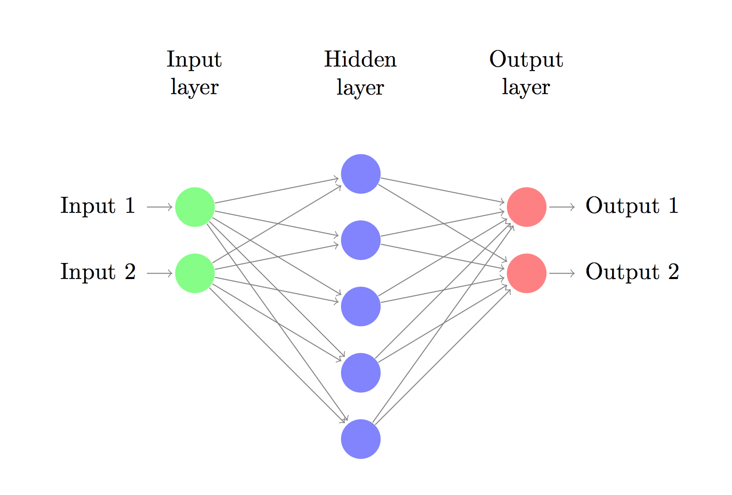
How to choose the size of the hidden layer? While there are some general guidelines and recommendations, it always depends on your specific problem and is more of an art than a science. We will play with the number of nodes in the hidden later later on and see how it affects our output.

神经网络的结构图

ReLu(Rectified Linear Units)激活函数

the softmax function, or normalized exponential function

cross-entroy loss

classify C classes

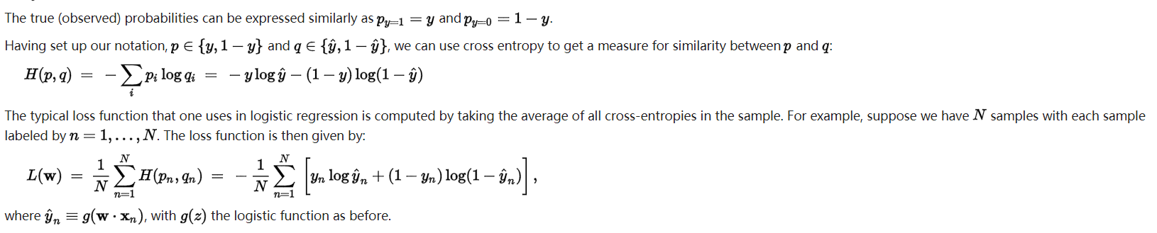
$L(y, y_hat) = - frac{1}{N} \sum_{n in N} \sum{i in C} y_{n,i} log y^{hat}\_{n,i}$ The formula looks complicated, but all it really does is sum over our training examples and add to the loss if we predicted the incorrect class. The further away the two probability distributions y (the correct labels) and \hat{y} (our predictions) are, the greater our loss will be. By finding parameters that minimize the loss we maximize the likelihood of our training data.

如果是logistic regression的话，

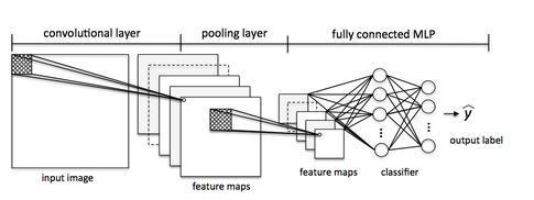
CNN的步骤：

The Convolution Step
Non Linearity (ReLU)
Pooling or Sub Sampling
Classification (Fully Connected Layer)

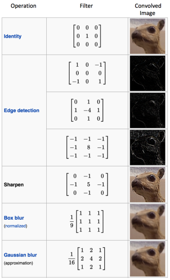
In CNN terminology, the 3×3 matrix is called a ‘filter‘ or ‘kernel’ or ‘feature detector’ and the matrix formed by sliding the filter over the image and computing the dot product is called the ‘Convolved Feature’ or ‘Activation Map’ or the ‘Feature Map‘. It is important to note that filters acts as feature detectors from the original input image.

It is important to note that the Convolution operation captures the local dependencies in the original image. Also notice how these two different filters generate different feature maps from the same original image.

In the table below, we can see the effects of convolution of the above image with different filters. As shown, we can perform operations such as Edge Detection, Sharpen and Blur just by changing the numeric values of our filter matrix before the convolution operation [8] – this means that different filters can detect different features from an image, for example edges, curves etc.

Sharpen: 0 -1 0 -1 5 -1 0 -1 0

Blur: 1 1 1 1 1 1 1 1 1

Edge enhance 0 0 0 -1 1 0 0 0 0

Edge detect 0 1 0 1 -4 1 0 1 0

Emboss -2 -1 0 -1 1 1 0 1 2

The more number of filters we have, the more image features get extracted and the better our network becomes at recognizing patterns in unseen images.

The size of the Feature Map (Convolved Feature) is controlled by three parameters that we need to decide before the convolution step is performed

Depth: number of filters
Stride: Stride is the number of pixels by which we slide our filter matrix over the input matrix. (移动的步长)
Zero-padding: Sometimes, it is convenient to pad the input matrix with zeros around the border, so that we can apply the filter to bordering elements of our input image matrix. A nice feature of zero padding is that it allows us to control the size of the feature maps. Adding zero-padding is also called wide convolution, and not using zero-padding would be a narrow convolution. This has been explained clearly in [14].

ReLU stands for Rectified Linear Unit and is a non-linear operation. ReLU output = max(0, input)

ReLU is an element wise operation (applied per pixel) and replaces all negative pixel values in the feature map by zero.

ReLU is an element wise operation (applied per pixel) and replaces all negative pixel values in the feature map by zero. The purpose of ReLU is to introduce non-linearity in our ConvNet, since most of the real-world data we would want our ConvNet to learn would be non-linear (Convolution is a linear operation – element wise matrix multiplication and addition, so we account for non-linearity by introducing a non-linear function like ReLU).

ReLU operation用在哪一步？

The Pooling Step

Spatial Pooling (also called subsampling or downsampling) reduces the dimensionality of each feature map but retains the most important information. Spatial Pooling can be of different types: Max, Average, Sum etc.

The function of Pooling is to progressively reduce the spatial size of the input representation [4]. In particular, pooling

makes the input representations (feature dimension) smaller and more manageable reduces the number of parameters and computations in the network, therefore, controlling overfitting [4] makes the network invariant to small transformations, distortions and translations in the input image (a small distortion in input will not change the output of Pooling – since we take the maximum / average value in a local neighborhood). helps us arrive at an almost scale invariant representation of our image (the exact term is “equivariant”). This is very powerful since we can detect objects in an image no matter where they are located

Fully Connected Layer

The Fully Connected layer is a traditional Multi Layer Perceptron that uses a softmax activation function in the output layer (other classifiers like SVM can also be used, but will stick to softmax in this post).

The output from the convolutional and pooling layers represent high-level features of the input image. The purpose of the Fully Connected layer is to use these features for classifying the input image into various classes based on the training dataset.

Apart from classification, adding a fully-connected layer is also a (usually) cheap way of learning non-linear combinations of these features

The overall training process of the Convolution Network may be summarized as below:

Step1: We initialize all filters and parameters / weights with random values
Step2: The network takes a training image as input, goes through the forward propagation step (convolution, ReLU and pooling operations along with forward propagation in the Fully Connected layer) and finds the output probabilities for each class. Lets say the output probabilities for the boat image above are [0.2, 0.4, 0.1, 0.3] Since weights are randomly assigned for the first training example, output probabilities are also random.
Step3: Calculate the total error at the output layer (summation over all 4 classes) Total Error = ∑ ½ (target probability – output probability) ²
Step4: Use Backpropagation to calculate the gradients of the error with respect to all weights in the network and use gradient descent to update all filter values / weights and parameter values to minimize the output error. The weights are adjusted in proportion to their contribution to the total error. When the same image is input again, output probabilities might now be [0.1, 0.1, 0.7, 0.1], which is closer to the target vector [0, 0, 1, 0]. This means that the network has learnt to classify this particular image correctly by adjusting its weights / filters such that the output error is reduced. Parameters like number of filters, filter sizes, architecture of the network etc. have all been fixed before Step 1 and do not change during training process – only the values of the filter matrix and connection weights get updated.
Step5: Repeat steps 2-4 with all images in the training set.

Also, it is not necessary to have a Pooling layer after every Convolutional Layer. As can be seen in the Figure 16 below, we can have multiple Convolution + ReLU operations in succession before having a Pooling operation.

Other ConvNet Architectures

AlexNet (2012) – In 2012, Alex Krizhevsky (and others) released AlexNet which was a deeper and much wider version of the LeNet and won by a large margin the difficult ImageNet Large Scale Visual Recognition Challenge (ILSVRC) in 2012. It was a significant breakthrough with respect to the previous approaches and the current widespread application of CNNs can be attributed to this work.
ZF Net (2013) – The ILSVRC 2013 winner was a Convolutional Network from Matthew Zeiler and Rob Fergus. It became known as the ZFNet (short for Zeiler & Fergus Net). It was an improvement on AlexNet by tweaking the architecture hyperparameters.
GoogLeNet (2014) – The ILSVRC 2014 winner was a Convolutional Network from Szegedy et al. from Google. Its main contribution was the development of an Inception Module that dramatically reduced the number of parameters in the network (4M, compared to AlexNet with 60M).
VGGNet (2014) – The runner-up in ILSVRC 2014 was the network that became known as the VGGNet. Its main contribution was in showing that the depth of the network (number of layers) is a critical component for good performance.
ResNets (2015) – Residual Network developed by Kaiming He (and others) was the winner of ILSVRC 2015. ResNets are currently by far state of the art Convolutional Neural Network models and are the default choice for using ConvNets in practice (as of May 2016).
DenseNet (August 2016) – Recently published by Gao Huang (and others), the Densely Connected Convolutional Network has each layer directly connected to every other layer in a feed-forward fashion. The DenseNet has been shown to obtain significant improvements over previous state-of-the-art architectures on five highly competitive object recognition benchmark tasks. Check out the Torch implementation here.

What is the difference between deep learning and usual machine learning?

One of the key ideas behind deep learning is to extract high level features from the given dataset. Thereby, deep learning aims to overcome the challenge of the often tedious feature engineering task and helps with parameterizing traditional neural networks with many layers.

Now, the problem with deep neural networks is the so-called “vanishing gradient” – the more layers we add, the harder it becomes to “update” our weights because the signal becomes weaker and weaker. Since our network’s weights can be terribly off in the beginning (random initialization) it can become almost impossible to parameterize a “deep” neural network with backpropagation.

Roughly speaking, we can think of deep learning as “clever” tricks or algorithms that can help us with the training of such “deep” neural network structures.

In applications of “usual” machine learning, there is typically a strong focus on the feature engineering part; the model learned by an algorithm can only be so good as its input data. Of course, there must be sufficient discriminatory information in our dataset, however, the performance of machine learning algorithms can suffer substantially when the information is buried in meaningless features. The goal behind deep learning is to automatically learn the features from (somewhat) noisy data; it’s about algorithms that do the feature engineering for us to provide deep neural network structures with meaningful information so that it can learn more effectively. We can think of deep learning as algorithms for automatic “feature engineering,” or we could simply call them “feature detectors,” which help us to overcome the vanishing gradient challenge and facilitate the learning in neural networks with many layers.

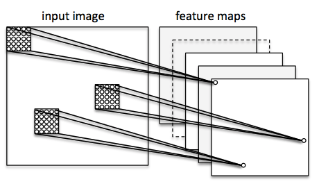
Let’s consider a ConvNet in context of image classification. Here, we use so-called “receptive fields” (think of them as “windows”) that slide over our image. We then connect those “receptive fields” (for example of the size of 5x5 pixel) with 1 unit in the next layer, this is the so-called “feature map.” After this mapping, we have constructed a so-called convolutional layer. Note that our feature detectors are basically replicates of one another – they share the same weights. The idea is that if a feature detector is useful in one part of the image it is likely that it is useful somewhere else, but at the same time it allows each patch of image to be represented in several ways.

Calculus on Computational Graphs: Backpropagation

Forward-mode differentiation tracks how one input affects every node. Reverse-mode differentiation tracks how every node affects one output. That is, forward-mode differentiation applies the operator ∂∂X∂∂X to every node, while reverse mode differentiation applies the operator ∂Z∂∂Z∂ to every node.1

When I say that reverse-mode differentiation gives us the derivative of e with respect to every node, I really do mean every node. We get both ∂e∂a∂e∂a and ∂e∂b∂e∂b, the derivatives of ee with respect to both inputs. Forward-mode differentiation gave us the derivative of our output with respect to a single input, but reverse-mode differentiation gives us all of them.

For this graph, that’s only a factor of two speed up, but imagine a function with a million inputs and one output. Forward-mode differentiation would require us to go through the graph a million times to get the derivatives. Reverse-mode differentiation can get them all in one fell swoop! A speed up of a factor of a million is pretty nice!

(Are there any cases where forward-mode differentiation makes more sense? Yes, there are! Where the reverse-mode gives the derivatives of one output with respect to all inputs, the forward-mode gives us the derivatives of all outputs with respect to one input. If one has a function with lots of outputs, forward-mode differentiation can be much, much, much faster.)

Backpropagation is also a useful lens for understanding how derivatives flow through a model. This can be extremely helpful in reasoning about why some models are difficult to optimize. The classic example of this is the problem of vanishing gradients in recurrent neural networks.

What do the fully connected layers do in CNNs?

The output from the convolutional layers represents high-level features in the data. While that output could be flattened and connected to the output layer, adding a fully-connected layer is a (usually) cheap way of learning non-linear combinations of these features.

Essentially the convolutional layers are providing a meaningful, low-dimensional, and somewhat invariant feature space, and the fully-connected layer is learning a (possibly non-linear) function in that space.

NOTE: It is trivial to convert from FC layers to Conv layers. Converting these top FC layers to Conv layers can be helpful as this page describes.

How is a CNN able to learn invariant features?

pooling operations are responsible for the translation invariant property in CNNs. I believe that invariance (at least to translation) is due to the convolution filters (not specifically the pooling) and due to the fully-connected layer.

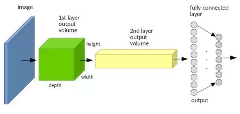
These volumes are build using a convolution plus a pooling operation. The pooling operation reduces the height and width of these volumes, while the increasing number of filters in each layer increases the volume depth.

The same number of activations occurs in this example, however they occur in a different region of the green and yellow volumes. Therefore, any activation point at the first slice of the yellow volume means that a face was detected, INDEPENDENTLY of the face location. Then the fully-connected layer is responsible to “translate” a face and two arms to an human body. In both examples, an activation was received at one of the fully-connected neurons. However, in each example, the activation path inside the FC layer was different, meaning that a correct learning at the FC layer is essential to ensure the invariance property.

It must be noticed that the pooling operation only “compresses” the activation volumes, if there was no pooling in this example, an activation at the first slice of the yellow volume would still mean a face.

In conclusion, what makes a CNN invariant to object translation is the architecture of the neural network: the convolution filters and the fully-connected layer. Additionally, I believe that if a CNN is trained showing faces only at one corner, during the learning process, the fully-connected layer may become insensitive to faces in other corners.

##关于backpropagation算法的理解

https://www.zhihu.com/question/24827633/answer/91489990

http://galaxy.agh.edu.pl/~vlsi/AI/backp_t_en/backprop.html

Logistic Regression和Neural Network对比

基础模型对比只有一层的Neural Network模型就是标准的Logistic Regression模型。神经网络就是由一个个逻辑回归模型连接而成的，它们彼此作为输入和输出。
多分类模型对比在逻辑回归中，决策边界由 θ’x=0 决定，随着参数项的增加，逻辑回归可以在原始特征空间学习出一个非常复杂的非线性决策边界（也就是一个复杂非线性方程）；　在神经网络中，决策边界由 ΘX=0 决定（这只是一个象征性表达式，Θ表示所有权重矩阵，X表示特征加上所有隐藏单元），其实神经网络算法并没有直接在原始特征空间学习决策边界，而是将分类问题映射到了一个新的特征空间，通过解决新特征空间的分类问题（学习决策边界），从而对应解决原始特征空间的分类问题。
性能对比如果给定基础特征的数量为100，那么在利用逻辑回归解决复杂分类问题时会遇到特征项会爆炸增长，造成过拟合以及运算量过大问题。例如，在n=100的情况下构建二次项特征变量，最终有5050个二次项。随着特征个数 n 的增加，二次项的个数大约以 n^2 的量级增长，其中 n 是原始项的个数，二次项的个数大约是 (n^2)/2 个。

而对于神经网络，可以通过隐层数量和隐藏单元数量来控制假设函数的复杂程度，并且在计算时只计算一次项特征变量。其实本质上来说，神经网络是通过这样一个网络结构隐含地找到了所需要的高次特征项，从而化简了繁重的计算。

ReLU激活函数的好处

作者：crackhopper 链接：https://www.zhihu.com/question/29021768/answer/43517930 来源：知乎著作权归作者所有。商业转载请联系作者获得授权，非商业转载请注明出处。

激活函数的作用：是为了增加神经网络模型的非线性。否则你想想，没有激活函数的每层都相当于矩阵相乘。就算你叠加了若干层之后，无非还是个矩阵相乘罢了。所以你没有非线性结构的话，根本就算不上什么神经网络。
为什么ReLU效果好：重点关注这章6.6节：Piecewise Linear Hidden Units(http://www.iro.umontreal.ca/~bengioy/dlbook/mlp.html)

总结如下：发现ReLU效果显著的论文： Jarrett, K., Kavukcuoglu, K., Ranzato, M., and LeCun, Y. (2009a). What is the best multi-stage architecture for object recognition?

发现ReLU更容易学习优化。因为其分段线性性质，导致其前传，后传，求导都是分段线性。而传统的sigmoid函数，由于两端饱和，在传播过程中容易丢弃信息： Glorot, X., Bordes, A., and Bengio, Y. (2011b). Deep sparse rectifier neural networks. In JMLRW&CP: Proceedings of the Fourteenth International Conference on Artificial Intelligence and Statistics (AISTATS 2011). 130,297

缺点是不能用Gradient-Based方法。同时如果de-active了，容易无法再次active。不过有办法解决，使用maxout激活函数： Goodfellow, I. J., Warde-Farley, D., Mirza, M., Courville, A., and Bengio, Y. (2013a). Maxout networks. In S. Dasgupta and D. McAllester, editors, ICML’13, pages 1319–1327. 130, 152, 243

除了帮助传播信息，便于优化的优点以外，分段线性函数可以让regularize变得更加容易。

作者：Begin Again 链接：https://www.zhihu.com/question/29021768/answer/43488153 来源：知乎著作权归作者所有。商业转载请联系作者获得授权，非商业转载请注明出处。

第一个问题：为什么引入非线性激励函数？

如果不用激励函数（其实相当于激励函数是f(x) = x），在这种情况下你每一层输出都是上层输入的线性函数，很容易验证，无论你神经网络有多少层，输出都是输入的线性组合，与没有隐藏层效果相当，这种情况就是最原始的感知机（Perceptron）了。

正因为上面的原因，我们决定引入非线性函数作为激励函数，这样深层神经网络就有意义了（不再是输入的线性组合，可以逼近任意函数）。最早的想法是sigmoid函数或者tanh函数，输出有界，很容易充当下一层输入（以及一些人的生物解释balabala）。

第二个问题：为什么引入Relu呢？

第一，采用sigmoid等函数，算激活函数时（指数运算），计算量大，反向传播求误差梯度时，求导涉及除法，计算量相对大，而采用Relu激活函数，整个过程的计算量节省很多。

第二，对于深层网络，sigmoid函数反向传播时，很容易就会出现梯度消失的情况（在sigmoid接近饱和区时，变换太缓慢，导数趋于0，这种情况会造成信息丢失，参见 @Haofeng Li 答案的第三点），从而无法完成深层网络的训练。

第三，Relu会使一部分神经元的输出为0，这样就造成了网络的稀疏性，并且减少了参数的相互依存关系，缓解了过拟合问题的发生（以及一些人的生物解释balabala）。当然现在也有一些对relu的改进，比如prelu，random relu等，在不同的数据集上会有一些训练速度上或者准确率上的改进，具体的大家可以找相关的paper看。

多加一句，现在主流的做法，会多做一步batch normalization，尽可能保证每一层网络的输入具有相同的分布[1]。而最新的paper[2]，他们在加入bypass connection之后，发现改变batch normalization的位置会有更好的效果。大家有兴趣可以看下。

[1] Ioffe S, Szegedy C. Batch normalization: Accelerating deep network training by reducing internal covariate shift[J]. arXiv preprint arXiv:1502.03167, 2015.

[2] He, Kaiming, et al. “Identity Mappings in Deep Residual Networks.” arXiv preprint arXiv:1603.05027 (2016).

Reference

https://ujjwalkarn.me/2016/08/11/intuitive-explanation-convnets/

http://www.wildml.com/2015/09/implementing-a-neural-network-from-scratch/

https://github.com/rasbt/python-machine-learning-book/blob/master/faq/difference-deep-and-normal-learning.md

http://andrew.gibiansky.com/blog/machine-learning/convolutional-neural-networks/

http://colah.github.io/posts/2015-08-Backprop/

http://blog.csdn.net/walilk/article/details/50278697

http://blog.csdn.net/walilk/article/details/50504393

Machine Learning笔记(一)